Projects

Shock response of a space structure42,486-DOF spacecraft component · 38 minutes → 0.2 seconds · calibrated intervals on shock response

A component of a space structure takes an impulse load. A heavy central mass sits on rigid links above a cylindrical shell, and behind a shock-absorption block sits essential equipment. The question after the event is whether the acceleration that reached that equipment stayed within survivable limits, and it has to be answered from a handful of monitored points, close to real time.

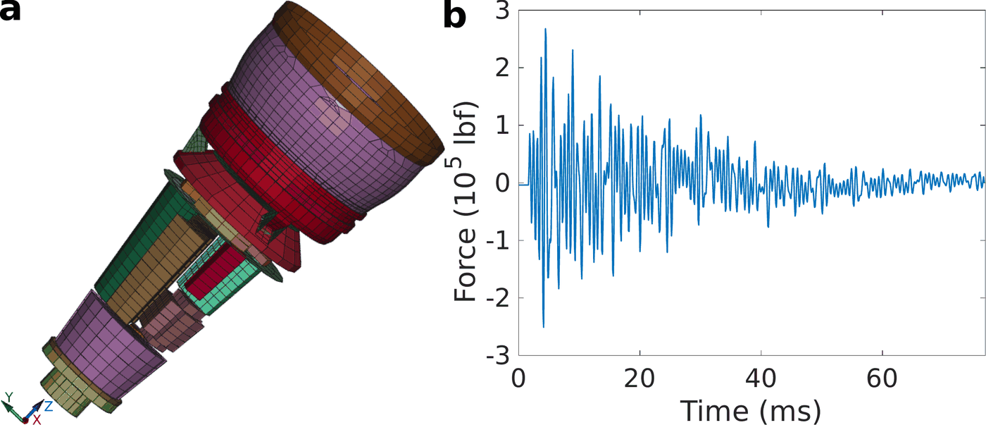
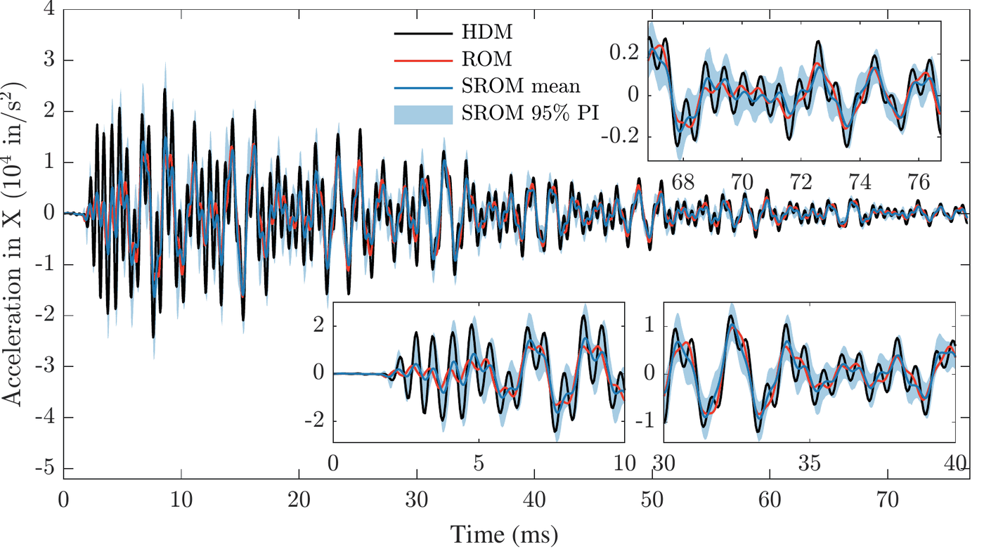
Left: the finite element model of the space structure component, showing the upper assembly, the cylindrical shell and the mounting pedestal. Right: the impulse force applied to the central mass, oscillating between plus and minus 2.5 times 10 to the 5 pound-force and decaying over roughly 75 milliseconds. — The component as modelled, and the shock it has to survive: the impulse decays over about 75 ms while exciting the full frequency content of the structure.

The high-fidelity finite element model that answers it has 42,486 degrees of freedom and takes about 38 minutes per run. A reduced-order model answers in 0.2 seconds, roughly 11,000× faster. That speedup is the only reason monitoring at this cadence is possible, and it is also what makes the answer untrustworthy: reducing the model discards the information needed to judge the result.

We made the fast model report its own reliability. Stochastic subspaces put the reduction error back into the prediction as a calibrated interval on acceleration and velocity at the critical nodes, and at nodes the fitting never saw. Bayesian optimization under uncertainty makes the calibration affordable at this scale, so the whole thing stays cheaper than the simulation it replaces.

Acceleration in X at a critical node over 75 milliseconds. The high-fidelity model is in black, the reduced-order model in dashed red, the stochastic reduced-order model mean in blue, and its 95 percent predictive interval as a shaded band. Three inset panels zoom into the early, middle and late response. The reduced model systematically understates the peaks, while the shaded interval covers the high-fidelity response. — Acceleration at a critical node. The reduced model (red) misses the peaks that decide whether the equipment survives; the interval (shaded) covers the high-fidelity response (black) instead of hiding the gap, at 0.2 s per evaluation rather than 38 minutes.

Model built in LS-DYNA; transient response integrated with Newmark-β. SS-PPCA · SS-Bootstrap · BO under uncertainty

Calibrated forecasting with scientific foundation modelsFrozen pretrained backbones · uncertainty without retraining · evaluated on ClimaX

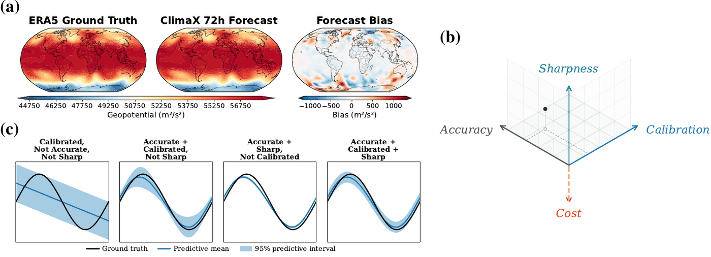
Pretrained foundation models are being adopted as general-purpose surrogates for weather and climate. ClimaX is one of them: a transformer trained on atmospheric data that produces forecasts far faster than numerical weather prediction, and produces them as single deterministic fields. A forecast without a credible spread cannot support a decision that depends on how bad the tail might be.

Panel a: ERA5 geopotential ground truth, the ClimaX 72-hour forecast, and the bias between them shown as global maps, with structured regional error. Panel b: axes for accuracy, sharpness and calibration, with cost pointing downward. Panel c: four schematic predictive bands illustrating that a model can be calibrated but not accurate, accurate but not sharp, accurate and sharp but not calibrated, or all three at once. — A 72-hour ClimaX forecast against ERA5, and the bias between them. The bias is structured, not random, which is what makes a single deterministic field inadequate and what a predictive interval has to account for. Accuracy, sharpness and calibration are separate properties: a model can have any two without the third.

The groups using these models generally cannot retrain them. The weights come from someone else, the compute to fine-tune them is not available, and the target system may have no training data at all.

We calibrate them from the outside. Resampling attention at inference turns a frozen backbone into a predictive ensemble whose spread tracks the errors it makes, with every pretrained weight untouched. Fine-tuned checkpoints work the same way, which matters because few groups deploy a foundation model straight out of the box.

Evaluated on pretrained atmospheric and time-series backbones. Calibrating Scientific Foundation Models with Inference-Time Stochastic Attention (under review)

Damage detection on steel truss bridgesDamage vs. seasonal temperature · likelihood-free inference · M.Tech thesis, IISc

A crack changes how a bridge vibrates. So does a twenty-degree change in air temperature, and it changes it by more. Any monitoring system that cannot separate the two will either raise alarms every summer or stay silent through real damage. The underlying inverse problem has no likelihood you can write down.

We used approximate Bayesian computation to infer damage state while treating thermal variation as part of the model rather than as noise to be filtered out, then extended it to the nonlinear response that damage itself introduces. This is where my interest in models that misreport their own confidence began.

M.Tech (Research) thesis, Indian Institute of Science, with Dr. Ananth Ramaswamy. Thesis · code · presented at ICCMS 2022, IIT Indore